Hunting for Insights: Investigating Predator-Prey Dynamics through Simulated Vision and Reinforcement Learning

Swiss Federal Institute of Technology Lausanne (EPFL)

Abstract

This study investigates how different vision fields affect predator-prey interactions. By simulating simplified environments and training agents with reinforcement learning, we observe trends that emerge in the strategies and effectiveness of trained predator and prey agents which use varying vision fields. Our findings support our current understanding that depth perception is very important for predators, whilst field of view is crucial for prey. Our work adds to existing literature regarding predator-prey simulations. By implementing some modifications to the setup, our approach enables exploring the complex interactions between predators and prey in novel ways.

I. Introduction

The natural world is full of fascinating and complex interactions between predators and prey, with each constantly adapting and evolving to survive. As researchers seek to better understand these dynamics, visual intelligence has emerged as a critical field of study, allowing us to gain new insights into how animals perceive and react to their environments.

In this work, we investigate the role of vision in prey-predator settings by leveraging reinforcement learning to train agents in simulated environments. Specifically, we are interested in how the field of view and the region of binocular vision affect the strategies and effectiveness used by predators and prey to hunt or evade respectively. We train predator and prey agents with varying vision fields in non-trivial environments with obstacles. The vision fields we experiment with are inspired by typical real-world predators and prey.

To evaluate the effectiveness of our approach, we both quantitatively evaluate agent performance in new environments and qualitatively observe the emergent strategies and behaviours of the agents under different configurations. Our work builds upon existing literature in this area to gain a deeper understanding of how differences in visual perception can influence predator-prey interactions.

The exploration of predator-prey dynamics in the context of vision has received relatively little attention in the existing literature. Research on simulated predator-prey systems commonly focuses on population dynamics and deals with very simple environments. At the same time, there have been major advancements in multi-agent reinforcement learning (MARL), making it possible to discover interesting group dynamics in complex environments. Given this, we present below some prior work related to this project.


Co-Evolution of Predator-Prey Ecosystems by Reinforcement Learning Agents [1]

This paper explores the use of MARL techniques to simulate the co-evolution mechanisms in predator-prey ecosystems. The study demonstrates a biologically plausible approximation of the agents' co-evolution over multiple generations in nature.

Comparison of potential distance metric that correlate with reachability.
Left: Initial random location of predators and prey.
Right: Emergence of swarming among predators and prey.

However, this work is limited to a simplified 2D environment without incorporating vision.

Emergent Tool Use from Multi-Agent Autocurricula [2]

Research conducted by OpenAI investigates the emergence of sophisticated tool use and coordination among agents in a hide-and-seek game environment, which shares similarities with predator-prey interactions. The study showcases the potential of multi-agent self-play in generating emergent auto curricula. Notably, this work trains agents in a complex environment equipped with vision sensors.

OpenAI Hide and Seek
Use of vision sensors in the hide-and-seek environment

However, this study does not explicitly explore the effects of varying the vision fields on the emergent behaviours of the agents.


Given the existing gaps in the literature for the study of predator-prey dynamics in the context of vision, our work aims to address them by incorporating various vision fields to represent different predators and prey. Through this approach, we investigate the impact of diverse visual perspectives on the emergent behaviours of the agents, providing valuable insights into the adaptive strategies employed in predator-prey interactions.

III. Methodology

In this section, we present the methodology utilized for this paper. We first discuss the environment setup, after which we detail how the predator and prey agents are created. Finally, we talk about how the agents are optimized.

We create a 3D environment using the Unity game development engine [3]. The selection of Unity as the engine for creating the environment instead of a different simulator is motivated by several key factors. Mainly, Unity's ML-Agents package [4] offers support for the OpenAI Gym framework [5], which is widely used in reinforcement learning research. This way, Unity enables interaction between the environment and the learning algorithms, allowing for efficient experimentation and evaluation of predator-prey agents.

Moreover, the engine offers a wide range of built-in tools, such as physics simulations, ray tracing, and collision. Finally, Unity provides a user-friendly and intuitive development environment, making it accessible to researchers with varying levels of expertise.

III-A. Environments

We present a diverse set of simulated environments aimed at replicating various scenarios involving predator-prey interactions. Our objective is to uncover a wide range of behaviors for the predators and prey. To achieve this diversity, we incorporate obstacles such as trees and rocks within the environments. Additionally, we introduce walls along the boundaries to confine the agents to the designated training area. This confinement allows us to concentrate the actions of an agent and observations within a controlled environment.

Furthermore, we integrate physics-based simulations and collision detection mechanisms into the environment. By assigning colliders to the predator and prey agent models, we ensure accurate detection of interactions with the environment and other agents. Each object in the environment is assigned a corresponding tag, such as "obstacle", "predator", or "prey", enabling efficient identification.

To speed up the learning process, we design the initial training environment ('Control' shown below) to be free of obstacles. This approach eliminates potential obstructions that could slow down training progress in the early stages. Subsequently, we create three additional training environments ('Forest', 'Escape Room' and 'Rocky') featuring distinct obstacle types: small trees, large rocks, and a split doorway. These environments allow the agents to acquire the skills necessary for navigating through increasingly complex situations involving obstacles, and should allow the prey agent to learn to exploit occlusions.

Environments used for training the agents

III-B. Predator and Prey Agents

Whilst the prey and predator have opposing objectives, they share similar characteristics. Both agents operate within a continuous action space with two degrees of freedom: rotation about the \(y\)-axis and forward/backward movement. Each degree of freedom allows the agent to select a value between \([-1, 1]\), determining the direction and intensity of movement. The agents' behavioural parameters consist of maximum movement and rotation speeds, which scale this intensity 
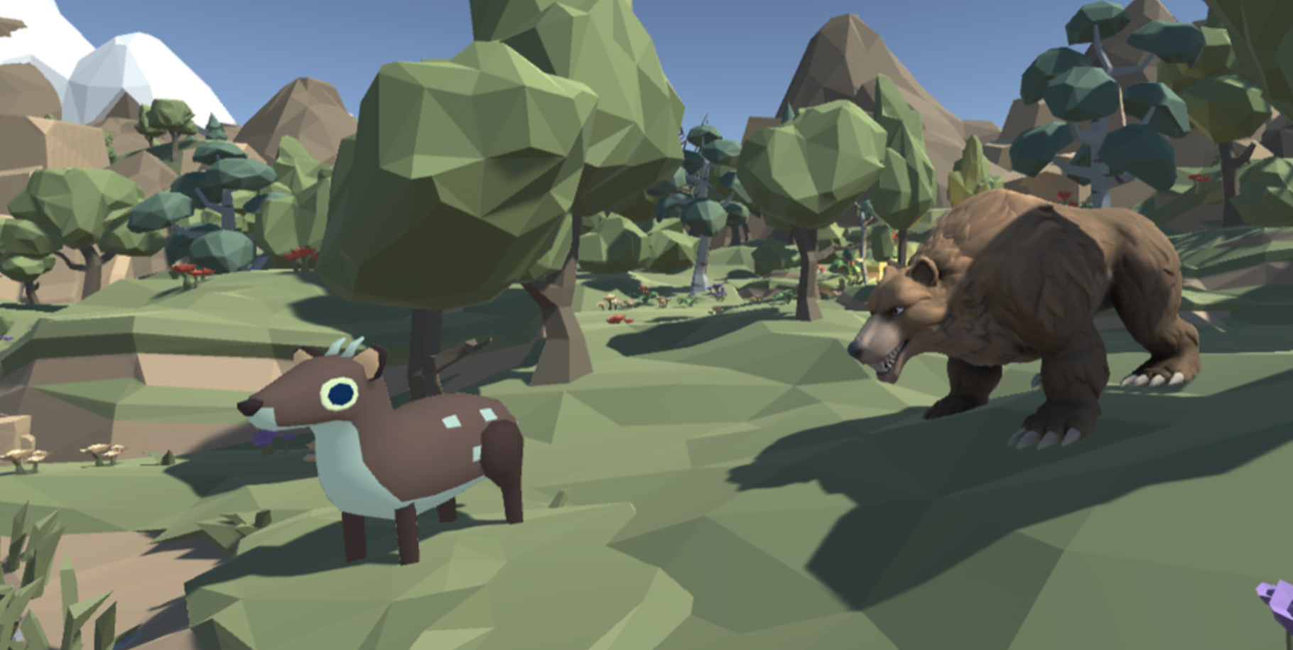
value. Notably, the predator possesses an additional box collider located at its face, resulting in the prey's death upon collision. Conversely, the prey lacks this collider as its primary goal involves evading the predator.


Box colliders for the agents
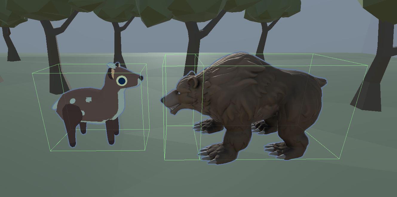
Box colliders for the predator and prey agents

Vision sensor

In order to simulate various vision fields, we employ a modified version of the ML-Agents Ray Perception sensor. This sensor uses a collection of ray casts originating from a central point. Several parameters are available to manipulate the vision, including ray angles (to establish the field of view), ray length (to determine the depth of field), number of rays (to regulate ray density/resolution), and a list of tags for filtering detected objects. Each ray conveys the following information: a flag indicating whether it collided with a tagged object, a one-hot encoded vector identifying the object type, and the normalized distance to the hit object relative to the ray length. Consequently, the sensor's output comprises a flattened vector encapsulating the information encoded within each ray.

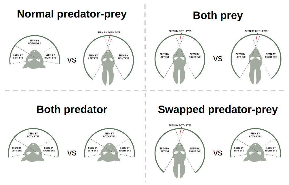
To control the region of binocular vision, we have extended this sensor to incorporate a parameter representing the number of depth rays. We make the simple assumption that agents can see the presence and type of an object across their entire field of view, but only have depth perception in their binocular region. Consequently, we exclude depth information for any rays falling outside this region by 
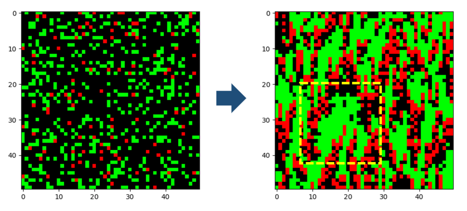
assigning a distance of \(-1\). Using this modified Ray Perception sensor, we define two distinct sensor types: predator-style and prey-style, which draw inspiration from the characteristic vision traits observed in real-world predators and prey [16], respectively.


Predator and prey-style ray perception sensors
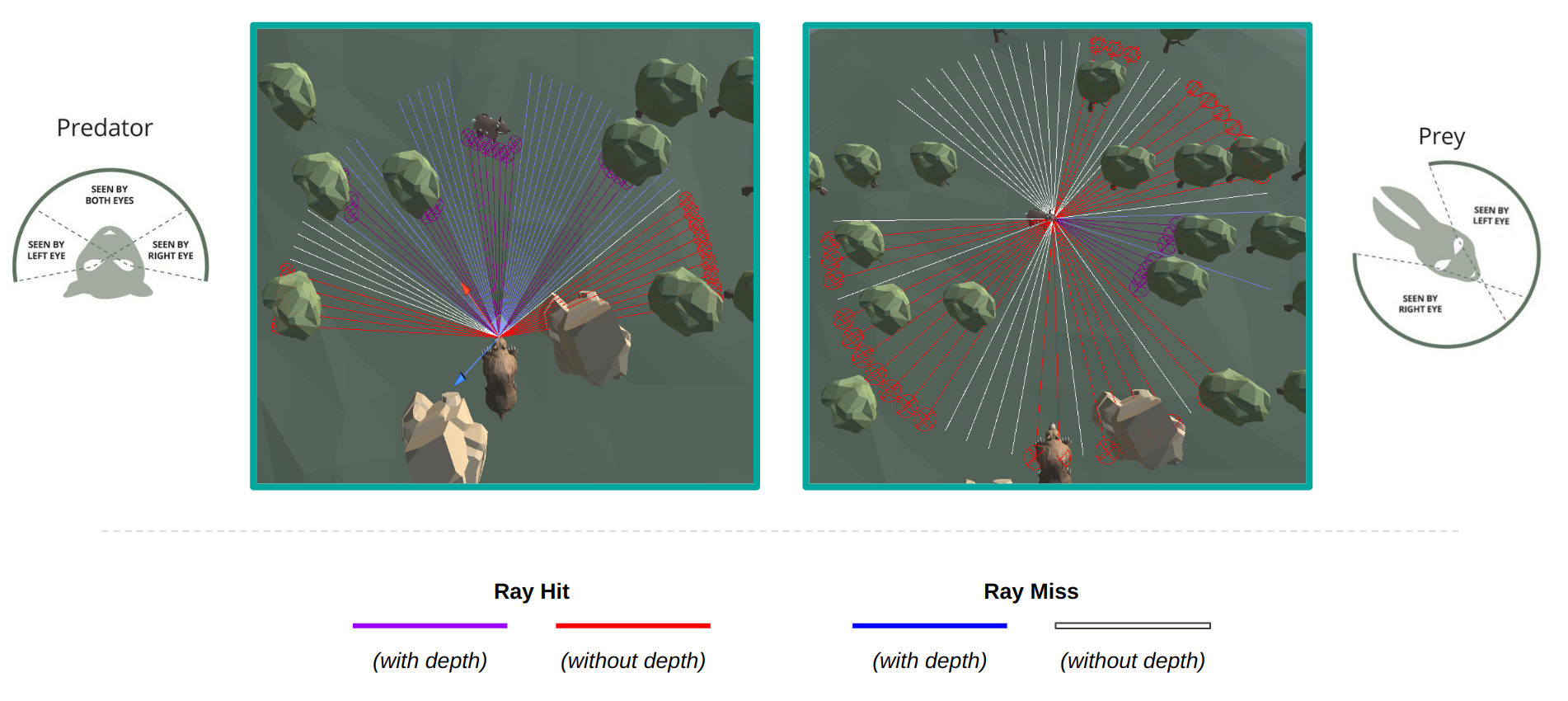
Predator- and prey-style ray perception sensors

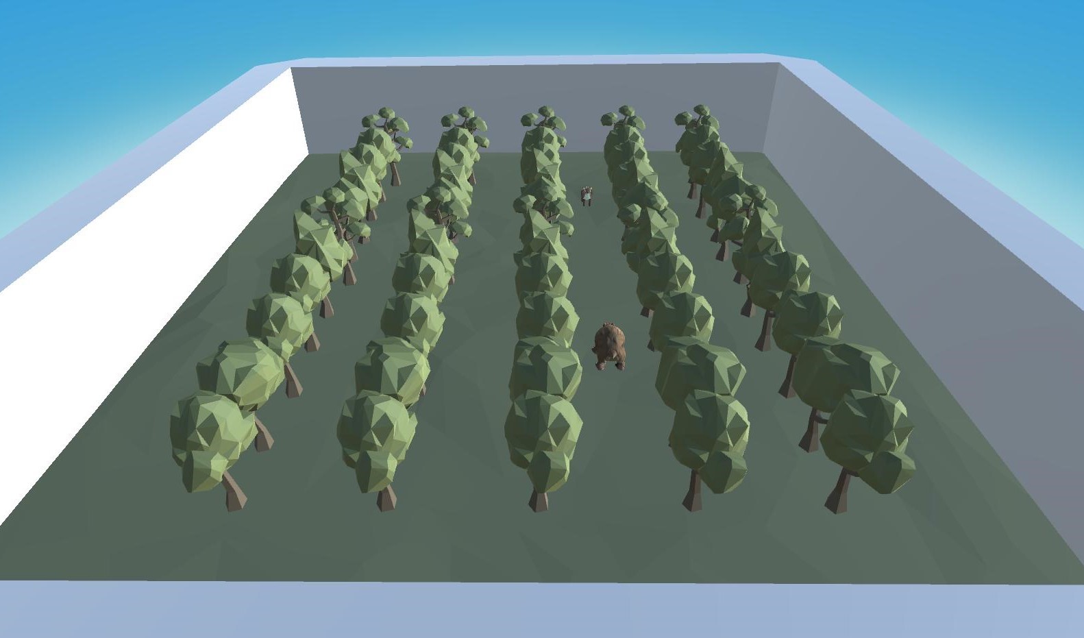
Utilizing the modified Ray Perception sensor offers distinct advantages for this paper by providing precise control over the simulated vision fields. Customizable parameters such as field of view and depth of field enable alignment with the specific requirements of the prey and predator agents in the simulated environment. This level of control ensures that the sensory input accurately reflects the desired characteristics of the vision of the agent. Furthermore, using the modified Ray Perception sensor instead of raw camera inputs enhances training efficiency by reducing the computational burden of processing high-dimensional image data.


III-C. Setting up Reinforcement Learning Training

The setting of predator-prey dynamics can be framed as a two-player dynamic game [6], [7]. This formulation captures the interactions and influence of the agents on the state of the game, providing a framework for studying predator-prey dynamics based on a common utility function. The game is only played for a set number of steps, until it is terminated.

In our formulation, the state and action spaces align with the descriptions provided in the previous sections, allowing for a consistent representation of the game dynamics. The transitions between states are determined by the underlying physics engine, ensuring a realistic simulation of the predator-prey environment.

$$ G_\text{pred} = \sum_{i=1}^{T}\left[\frac{𝟙(\text{prey caught at } t)}{N_\text{prey}} - \frac{1}{T}\right] $$ $$ G_\text{prey} = - G_\text{pred} $$

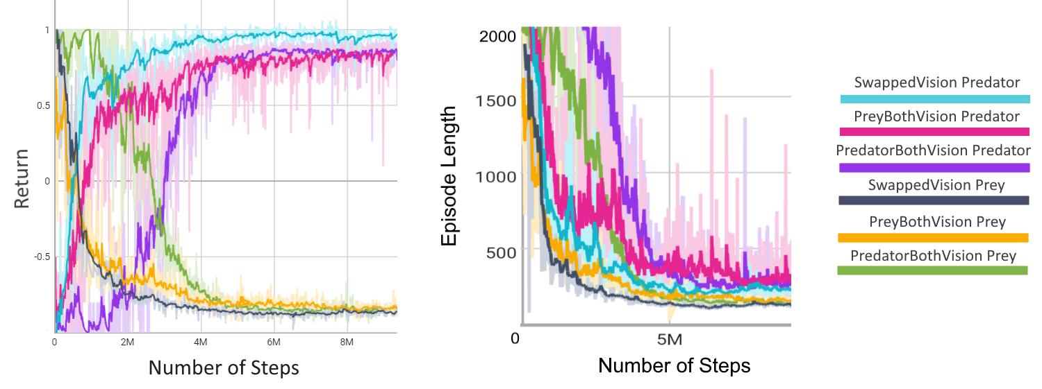
The reward structure employed in our proposed framework, as illustrated in the figure above, incorporates a constant time penalty applied to the predator at each time step, and a positive reward if a prey is caught. This deliberate design choice serves to incentivize the predator to capture prey at the earliest opportunity. Conversely, the reward for the prey is formulated in the opposite manner, establishing a zero-sum game. The range of rewards is bounded within the interval \([-1, 1]\). This reward specification enables a natural distinction between favorable and unfavorable outcomes of both agents.

Furthermore, since the predator-prey game exhibits an inherent asymmetry, it can be expressed as an asymmetric zero-sum game. Unlike games such as soccer, where teams have shared objectives, the predator and prey agents pursue conflicting goals. The asymmetry arises from the distinct policies used by the different agents, resulting in strategic dynamics that differ from those observed in symmetric games.

Overall, the nature of the game poses additional challenges, as it suffers from many of the problems in competitive multi-agent learning [8]. Multi-agent reinforcement learning in competitive scenarios poses several challenges [9]. In this paper, we employ a prominent technique called "self-play" [10], [11] to address these difficulties. The diagram below provides a high-level overview of this approach.


Self play
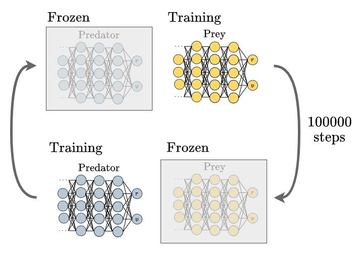
Diagram showing the self-play mechanism

Initially, either the predator or prey agent is trained, while the model of the other agent remains frozen. After a predetermined number of iterations, the frozen model is trained, and the other agent's model is frozen. However, a potential issue arises from the bias introduced by repeatedly playing against the most recent model. This bias can lead to overfitting and poor generalization. To mitigate this problem, we incorporate an ELO ranking system as done in MuZero [12], enabling models to compete against earlier versions of their opponents. By doing so, we reduce the impact of bias, leading to improved generalization and robustness in the learned policies.


IV. Experiments

In this section, we discuss the setup and results of the experiments in detail. Regarding results, we first discuss the training progression, after which we do both a qualitative and a quantitative analysis of the different agent configurations.


IV-A. Experimental Setup


Agent parameters

Rays per direction Depth rays per direction Max ray degrees Ray length Observation stacks Field of view Binocular region Maximum movement speed Maximum rotation speed
Prey-style 30 4 160 15 5 320° 43° 8 8
Predator-style 30 20 85 15 5 170° 113° 6 2
Parameters of the prey and predator-style vision sensors, and the behavioural parameters used for the agents.

Firstly, we establish two distinct categories of vision: prey-style and predator-style. This can be seen in the table above. Prey-style vision emphasizes a broad field of view while limiting the binocular region, whereas predator-style vision exhibits the opposite characteristics. Additionally, for both agents we stack the observations to simulate a brief memory of recent events.

During inference, we designate the maximum speed of the prey to be greater than that of the predator. We adopt this approach to give the prey a better chance to play out its learned strategies rather than getting caught too quickly in each episode.

Vision sensor configurations
The combinations of vision sensors used for the predator and prey in the experiments.

As depicted in the figure above, we train agents in \(4\) configurations to cover each combination of vision types for the predator and prey. The trained models are then used to perform inferences.

Training details

The agents are trained on all environments mentioned in the methodology section in parallel, using the parameters mentioned in the agent parameters section. The only difference is that the maximum speed of the prey was set to \(5.5\). By having environments of different difficulties, a speed-up in training can be observed, similar as in curriculum learning [13], [14]. Furthermore, three agents of each type were present in each environment. Although this could make the environment unstable due to partial observability, it greatly enhances training speed.

The predator and prey were each trained self-play for \(9 \cdot 10^6\) steps, where one step corresponds to one frame in the simulation. The swap between the frozen training teams happens every \(3 \cdot 10^5\) training steps. At each episode, the agent is spawned with a random rotation the y-axis, and the maximum episode duration is \(10^4\). The model plays against the most recent version of the agent \(80\%\) of the time. The models both consist of a \(3\) hidden-layer MLP with \(512\) neurons with batch normalisation at each layer. The model is optimized using PPO with the Adam [15] optimizer with a learning rate of \(0.0003\) and no decay. Finally, the buffer sizes of both agents are set to \(40960\).

Inference environments

For testing the agents we design new out of distribution environments with varying levels of complexity. The control environment, like in training, consists of an empty environment. Additional environments include similar obstacles and hiding spots in different configurations, introducing more blind spots for the prey to utilize for protection. The inference environments are shown below.


Environments used for inference

Hardware

The models were trained using a CUDA-enabled NVIDIA V100 PCIe \(32\) GB GPU with \(7\) TFLOPS, a Xeon-Gold processor running with a \(2.1\) GHz clock speed, and \(16\) GB of RAM. Our method is implemented with Unity’s ML-Agents package and PyTorch, running on Linux with Python 3.7.

IV-B. Results

Training results

Reward plot during training
(Left) Average returns over \(9\) million steps of training for each agent configuration. (Right) Average episode lengths over \(9\) million steps of training for each agent configuration. Note that, unfortunately, the training logs for 'Normal' vision were lost. However the trend in rewards was similar to the other plots shown here. Furthermore, take note that the x-axis represents the number of steps, so if the predator was trained first, it would swap at the step \(300000\), and the x-label for the prey at total step \(300005\) would be \(5\). An exponential smoothing of strength \(0.8\) is used.

The average returns during training for various vision configurations of predator and prey agents are illustrated in the left figure. It is observed that the PredatorBoth vision improves at a slower rate compared to other configurations, likely due to the reduced field of view when both agents have predator vision. However, this effect diminishes over time.

In the right figure, we analyze the episode length throughout the training process. Interestingly, we consistently observe a decreasing trend in episode length across all configurations. It is important to note however that whilst it may seem like the predator is learning to consistenly dominate the prey, the training environment is heavily biased towards the predator since there are three predators which can all catch the prey. Thus, to judge the true performance of the agents we perform inference in a more balanced environment.


Inference results

The plot below shows median number of steps survived by the prey in the inference environments for different configurations of vision sensors. We look at time survived in order to study the relative performance of each agent in different settings (higher time indicates more effective prey, lower time indicates more effective predator). We use median so that the results are not swayed by outliers which might be caused due to no interactions between the predator and prey, for example if they get stuck in an obstacle for an episode.


To comment further on the learned strategies of the agents under different configurations and to identify the reasons for the results we see above, we qualitatively assess some key behaviour patterns of the trained agents in each configuration.

Normal vision

This configuration features agents that are trained with their typical real-world vision field. We observe many instances that suggest both agents have learnt strategies to maximize their reward. The prey performs significantly worse with this configuration in the control environment, suggesting that it has learnt to effectively use obstacles in the other environments to evade the predator.

Predator: Chases the prey while trying to keep it in its binocular region. When the prey is in the monocular region it seems to favour rotation with slower movement speed, but when the prey is in its binocular region it makes bigger steps towards the prey. This likely hints at the importance of depth information for the predator, but it's possible that this is also influenced by the fact that the agents have very little memory (as evidenced by the predator forgetting about the prey as it falls out of its vision field), and is thus trying to simply keep the prey within its vision field for as long as possible.

Prey: As seen below, it has visibly learnt ways to evade the predators. It is able to keep track of the predator using its monocular vision and also uses obstacles to its advantage by either hiding behind or going around them. It also uses a zig zag motion to avoid the predator being in its blind spot.

Both predator

Since the prey is trained using predator-style vision, its blind spot is much larger, thus the prey is unaware if it is being chased from behind. It can only rely on cues ahead of it to keep track of objects and the predator.

Overall in this configuration there are also many instances which show that the prey has failed to properly learn to evade, even when the predator is directly in its vision field, indicating that these agents likely require further training.

Both prey

The median time survived by the prey is significantly higher across all environments in this configuration, indicating that the predator trained with prey-style vision is likely ineffective, whilst the prey is able to learn effetively.

Predator: Exhibits less aggressive behaviour and more tracking(in order to keep the prey in its narrow depth FOV) by rotating when the prey is in its monocular vision. The lower aggression exhbited by the predator is a major reason for longer median survival time of the prey.

Prey: We observe that the prey has learnt evasive strategies similar to the prey in the normal configuration. This can be seen in the video of the prey evading the predator in the control environment.

Swapped vision

This configuration has lower median time survived for the prey in all environments except control.

Prey: Exhibits behaviours suggesting that it has learnt to keep track of the predator in its frontal vision field and move backwards to run away from the predator. However since it is lacking a wide field of view, it is unware of the objects behind it and runs into them, making it an easy target. Thus the prey performs worse in environments with many obstacles (such as trees) and better in control which has no obstacles. In many examples it keeps backing up into the walls and corners until it is eventually caught by the predator. This is likely due to a lack of memory and positional information, which means that the agent doesn't realise that it's actions are futile and it's not moving anywhere.

Predator: Since it is trained on prey-style vision, it continues to rotate to try keep the prey in its binocular region, similar to the both-prey configuration. However since the prey is also less effective with predator-style vision, the predator has more success in this case with the median survival time for the prey being lower than the both-prey case (except for in control where the prey can be effective with predator-style vision).

V. Conclusions and Limitations

Our work investigates the role of vision in simulated predator-prey interactions. By varying the vision fields of predator and prey agents and training them using reinforcement learning, we make the following observations:

  • Depth information is crucial for predators, while prey also benefit from depth perception to a lesser extent.
  • Prey require a wide field of view to navigate while detecting predators in their periphery, whereas predators primarily look in the direction of their movement and thus don't require as wide a FOV.
  • Memory is crucial to visual perception in predator-prey interactions.
These observations support the understanding of why real-world predators prioritize depth perception and prey prioritize a wide field of view in their vision systems.

V-A. Limitations and Future Work

Although the initial results are promising, our approach has several limitations. Real-life predator prey interactions are incredibly complex, and it’s almost impossible to capture all these complexities in a simple simulated environment such as this. The most pertinent limitations and potential future work include:

  • The predator and prey agents sometimes displayed untrained or random behaviour, suggesting a need for further training. For comparison, OpenAI's hide and seek environment required ~\(2.7\) million episodes for seekers to consistently chase hiders, even with the aid of a curriculum learning approach. Our training lasted only around \(10\) million steps (order of magnitude of ~\(10^4\) episodes). Although training on OpenAI's scale is not feasible, additional training or alternative strategies such as curriculum learning could improve the agents.
  • Memory is crucial to complement vision in predator-prey scenarios, however our agents had virtually no memory. This, coupled with the lack of positional information to understand when they were stuck, greatly affected the agents performance. To address these issues, we could increase the observation stack to give the agents more memory, whilst including past positional information as an additional observation. Using a recurrent neural network instead of a vanilla multi-layer perceptron could also better model the temporal information.
  • Depth perception seems to play an important role for both predators and prey, but our simplified sensor assumes no depth perception outside of the binocular region which isn't strictly true. There are various monocular depth cues as well (as shown in the figure below) that both predators and prey in reality could make use of in their periphery. Thus, using a more complex sensor as such adding noisy depth estimates rather than no depth information in the monocular regions could help improve learning.
https://jackwestin.com/resources/mcat-content/perception/perceptual-organization
Examples of depth cues available from monocular vision
  • We simplified the action space for our agents by restricting them to backward/forward movement and rotation. In reality, predators and prey have more degrees of freedom, such as the ability to turn their heads and look in different directions while moving. This additional freedom, combined with memory, could for example provide advantages for prey with predator vision. They could look backward to assess the predator's location and then look forward again to escape, similar to how humans (who have predator-style vision) might behave when being chased.

Furthermore, in this initial work, we only investigate a discrete set of vision fields. However, a similar setup could also be used to instead optimise the vision fields for each agent's goal of evading/hunting, given some physical constraints.


Become the Predator

Play against a trained prey in our test environment by using your arrow keys. Please note that the predator has been slowed down, and you will likely easily be able to catch the prey. It is meant for getting an idea of the setup. The prey behaviour may not always be optimal, but if you play a few times you can start to observe some interesting behaviours.

References

  1. Park J, Lee J, Kim T, Ahn I, Park J. Co-Evolution of Predator-Prey Ecosystems by Reinforcement Learning Agents. Entropy. 2021; 23(4):461. https://doi.org/10.3390/e23040461.
  2. Baker, B., Kanitscheider, I., Markov, T., Wu, Y., Powell, G., McGrew, B., & Mordatch, I. (2019). Emergent tool use from multi-agent autocurricula. arXiv preprint arXiv:1909.07528.
  3. Haas, J. K. (2014). A history of the unity game engine.
  4. Juliani, A., Berges, V. P., Teng, E., Cohen, A., Harper, J., Elion, C., ... & Lange, D. (2018). Unity: A general platform for intelligent agents. arXiv preprint arXiv:1809.02627.
  5. Brockman, G., Cheung, V., Pettersson, L., Schneider, J., Schulman, J., Tang, J., & Zaremba, W. (2016). Openai gym. ArXiv Preprint ArXiv:1606.01540.
  6. Tsai, Dorian, Timothy L. Molloy, and Tristan Perez. "Inverse two-player zero-sum dynamic games." 2016 Australian Control Conference (AuCC). IEEE, 2016.
  7. Başar, T., & Olsder, G. J. (1998). Dynamic noncooperative game theory. Society for Industrial and Applied Mathematics.
  8. Buşoniu, L., Babuška, R., & De Schutter, B. (2010). Multi-agent reinforcement learning: An overview. Innovations in multi-agent systems and applications-1, 183-221.
  9. Shoham, Y., Powers, R., & Grenager, T. (2003). Multi-agent reinforcement learning: a critical survey (Vol. 288). Technical report, Stanford University.
  10. Bai, Y., Jin, C., & Yu, T. (2020). Near-optimal reinforcement learning with self-play. Advances in neural information processing systems, 33, 2159-2170.
  11. Silver, D., Hubert, T., Schrittwieser, J., Antonoglou, I., Lai, M., Guez, A., ... & Hassabis, D. (2018). A general reinforcement learning algorithm that masters chess, shogi, and Go through self-play. Science, 362(6419), 1140-1144.
  12. Schrittwieser, J., Antonoglou, I., Hubert, T., Simonyan, K., Sifre, L., Schmitt, S., ... & Silver, D. (2020). Mastering atari, go, chess and shogi by planning with a learned model. Nature, 588(7839), 604-609.
  13. Bengio, Y., Louradour, J., Collobert, R., & Weston, J. (2009, June). Curriculum learning. In Proceedings of the 26th annual international conference on machine learning (pp. 41-48).
  14. Narvekar, S., Peng, B., Leonetti, M., Sinapov, J., Taylor, M. E., & Stone, P. (2020). Curriculum learning for reinforcement learning domains: A framework and survey. The Journal of Machine Learning Research, 21(1), 7382-7431.
  15. Kingma, D. P., & Ba, J. (2014). Adam: A method for stochastic optimization. ArXiv Preprint arXiv:1412.6980

  16. Land, M. F., & Nilsson, D. E. (2012). Animal eyes. OUP Oxford.